Overview
In embedded techniques, we employ modeling algorithms that use the coefficients of features to minimize the number of features they have. Embedded techniques are one of the most advanced feature selection methods because they blend the advantages of filters or wrapper methods.
Process of Embedded Methods
In order to implement embedded methods, we must include features that are in the same order. It can be concluded that the features with the highest coefficients within the model are those which are significant and have an impact on our dependent variable. Likewise, the features that aren’t correlated to the output variable will have coefficients close to zero. But, it’s not as easy since each feature affects the output variable. If the quantity of features is too high, the size of the coefficients increases, making it difficult to discern which features are crucial and which aren’t. This is why we employ regularized models with an inbuilt function to regulate the dimension of the coefficients.

It is suggested to take the time to read Linear Regression to comprehend the information listed below.
There are two kinds of embedded methods: Lasso Regression (uses L1 regularization) and Ridge Regression (uses regularization using L2), which are Regularized Linear models employed to select features.
Ridge Regression
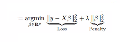
Ridge Regression can be used to build an ad hoc model in which constraints are included in the algorithm to penalize the coefficients that are too big and prevent them from getting overly complicated and leading to overfitting. In layman’s language, it adds an additional penalty to the equation, where w is the vector of coefficients for the model, which is the L2 norm and is a tunable free parameter. This makes the equation appear like this:

In this case, the first component is the term with the lowest square (loss function), and the second is penal. The Ridge Regression L2 regularization process is performed, which adds penalties equal to the size of the coefficients. So, under Ridge regression, the L2 norm penalty, which can be described as ani=1w2i, is added to the loss function, thereby penalizing betas. Since the coefficients are squared in the penalty function, this differs from an L1-norm that we employ to calculate Lasso Regression (discussed below). The alpha has a significant part in this as its value of it is determined in accordance with the model you wish to explore. So if we choose alpha as 0, it becomes Ridge, and alpha = 1. will be LASSO, and anything that falls between 0 and 1 is known as Elastic net.

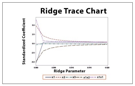
The next step is the most important aspect of the equation: choosing the value of the parameter that can be tunable Lambda. If we select a small lambda number, the result will be exactly that of the OLS Regression so that the generalization won’t occur. However, if we use too large of a lambda number, it will broaden excessively, reducing the coefficients of many features toward extreme minimal values (i.e., towards 0). Statistics employ methods like Ridge Trace, which is a diagram that illustrates the coefficients of ridge regression as a function of lambda. We choose the lambda value that stabilizes the coefficients. We can employ methods such as cross-validation, along with grid searches, to identify the optimal lambda to fit our model.

Ridge utilizes L2 regularization, which forces coefficients to be spread more evenly. It does not cause any coefficient to shrink to the point that it’s zero; however, L1 regularization forces the coefficients of less significant aspects to zero, leading to that Lasso Regression.
Note that Ridge Regression can be seen as a Method of Feature Selection method because it reduces the magnitude of coefficients and, unlike Lasso, does not render any of the variables obsolete, which could be considered a valid feature Selection method.
Lasso Regression
Lasso is the same as Ridge; however, it performs L1 regularization, which introduces the cost ani=1|wi| to the loss function, resulting in a penalty equal to absolute values of coefficients, not that of their squares (used to calculate L2) that causes weaker features to have zero coefficients. By making use of L1 regularization, Lasso does an automatic feature selection process, where features with zero as their coefficients are removed. Also, the lambda value is vital because if its value is too large, it can result in dropping many variables (by making the coefficients that are a small change to zero), rendering the model too general, and causing the model not to be able to fit.

If we use the right value for lambda, we can produce a light output, where certain features that are not important are listed with coefficients of 0. These variables can be removed, and those with non-zero coefficients may be chosen, thereby facilitating the selection of features for modeling.
These models, which are regularized, are able to identify the right relationship between dependent and independent variables by regularizing the dependent variable’s coefficient. They can help reduce the threat of multicollinearity. Regularization of certain regression models could be difficult if the independent features are not linearly connected to the dependent variable. To address this issue, we can alter the features to ensure that linear models like Ridge and Lasso are still applicable, like applying polynomial basis functions to linear regression. These transformed features enable the model’s linearity to discover the polynomial or non-linear relationships within the data.


