Overview
Hypothesis Testing is among the most essential aspects of Inferential Statistics. As discussed in the “descriptive Statistics” section, various descriptive statistics are used to describe the data simply. However, using statistical inference, we attempt to draw a conclusion. with hypothesis testing, we attempt to determine if an event that occurs in a particular population is actually observed in the general population as well and, if it is the case, if it isn’t, how certain can we be in either the assertions or attempt to evaluate the results and formulate a hypothesis, what can we say regarding this Hypothesis? For all of this, we can conduct the hypothesis test so that we are able to reject the Hypothesis or agree with it. The hypothesis is an inference that connects one independent and dependent. There are many kinds of testing hypotheses for various situations. Some of the most crucial hypothesis tests are listed below.

These Hypothesis tests are extremely beneficial because they give exact and precise responses to our specific questions.
Null and Alternative Hypothesis Testing
Each Hypothesis test is conducted to determine whether or not to accept the Null Hypothesis.
Null Hypothesis Testing
The definition of the term null Hypothesis may differ for every type of Hypothesis Testing and is also dependent on the particular issue; however, more or less, The Null Hypothesis generally implies that there is no proof of any effect, i.e., in the case of comparing a sample’s mean with the average of the population. The Null hypothesis would be that both means are equivalent to one another.
H0: m = x
Alternative Hypothesis Testing
The Alternate Hypothesis is the reverse of that of the Null Hypothesis Testing. It declares that the mean of the sample may be greater or less than the mean of the entire population or, in other words, that the mean of the population does not correspond to the sample mean.
H1: m x
Two-Tailed, One-Tailed Hypothesis Testing
Two-Tailed
Sometimes, the alternative theory simply states that the mean of the sample isn’t the same as the mean of the entire population. This is referred to as a Two-Tailed Test, also known as a Non-Directional, because we don’t specify an exact ‘direction’ to the Hypothesis. This is why the alternate Hypothesis will be rejected when the sample’s mean isn’t equivalent to the population’s mean because the sample is too big or too small compared to the population’s mean. An Alternative Hypothesis Testing is formulated when the researchers aren’t sure of the possibility that the result could be positive or negative.
One-Tailed
On the other side, the Directional, aka One-Tailed Hypothesis, is when we establish the alternative Hypothesis that we’re interested in, such as if we’re just looking to determine whether the mean of the samples is higher than the general mean of the population or not. In this case, a lower value or, for instance, a decrease in the mean of the sample is not of any value to us. Therefore we set our Alternative Hypothesis as
H1: m < x
Types of Error
Researchers could make two kinds of mistakes while conducting the hypothesis test: the Type I error and then Type II.
Type I Error
Rejecting Null Hypothesis when it could be accepted.
Type II Error
Accepting a Null Hypothesis in the event that it should have been rejected.
A few of these mistakes can result in a very incorrect interpretation of data, and the errors must be avoided at all costs.
P Value, Significance Level, and Confidence Level
P Value
We utilize the value of p to decide whether or not to accept an unproven hypothesis. Based on p-values, we can determine what the significance of the “change. It is the most fundamental and essential element of any Hypothesis Test and must be fully understood to avoid Type I and II errors. In simple words, the p-value is the value of the test.
- The probability of obtaining the observed or more significant results when the null hypothesis is valid.
- The probability of a statistical model, if the null hypothesis holds, is that the summary of statistical data (such as the mean of the sample differences between two groups) will be similar to or larger than the actual observed results.
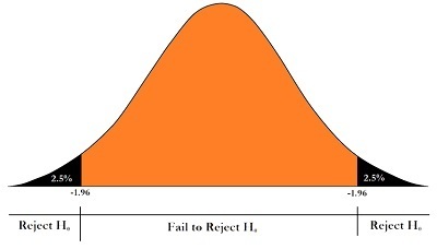
Significance Level
Significance Level: significance level (symbolized as an (alpha) It is used to indicate the probability we use to decide whether to admit the non-truth Hypothesis. We calculate the p-value. Based on our “cut-off” or Significance threshold, we either accept or reject our Null Hypothesis Testing. For instance, the Significance Level we have set is 5%. When we set the significance level at 5%, we are referring to the probability of receiving our measured value (e.g., the sample mean) as less than 5 per cent. If the p-value is found out as, e.g., 0.04 (4 per cent), the likelihood of randomly getting the number we tested (e.g., mean of the sample) is lower than 4%. This allows us to believe that the number we received is not a result of chance since the likelihood of obtaining such numbers randomly is as low as the per cent. According to our significance level, if our probability of receiving a number via random chance falls below 5%, we can conclude that the change in our mean for our sample can be considered statistically significant. If we had set the significance threshold at 1%, then the number of sample p-values would have made us conclude that the amount that we got was a result of random chance and not a result of random sampling. For our sample significance, the p-value has to be lower than 0.01, i.e., less than 1 per cent. The significance degree is highly individual and can be influenced by the needs of the particular business or the particular domain.
Confidence level
The confidence level is simply 1-Significance level, i.e., If our significance is set at 5%, our Confidence level will be 95%. If our p-value turns out to be 0.04 and we are able to be 96% certain that our sample’s average is not due to randomness or chance but rather reflects a variation of the median.
In general, the significance level is set at 5 percent. The value of p (P) generally refers to
- P > 0.05 statistically insignificant (more than one out of 20 probability of being incorrect)
- P 0.05 is significantly significant (less than 1/20 probability of being incorrect)
- P 0.01 statistically significant (less than one out of 100 chances of being incorrect)
- P 0.001 statistically relevant (less than one in thousand chance of being right)
In order to use the p-value in Accepting or Rejecting this Null Hypothesis Testing, it’s crucial to keep in mind that if the p-value of our sample is lower than the selected significance level, then we will do not accept our Null Hypothesis, i.e., accept that the value of our sample (e.g., the mean of our sample) is solid evidence in support of the Hypothesis of alternative.
One method to remember this is to recall phrases. One of the phrases that can be used to remember is:
“If P is low, Null will go. If P is high, then Null will decide.”
It’s an extremely intuitive way to remember; however, sometimes, it can be helpful if we set the significance value as 55%. If the p-value is very low (lower than 0.05 marks), we deny this Null Hypothesis (Null can decide where it will decide and will not be used). If the value for p is excessive (higher than the 0.05 value), then we agree with the Null Hypothesis (Null can make the final decision and be utilized to draw the inference).
Examples
For a better understanding of the significance and p-value of p-values and Confide Level, three examples will be included to understand better. In Examples 1 and 2, the alternative Hypothesis will be directional, whereas, in Example 3, the alternative Hypothesis will be non-directional.
Example 1
First, let’s look at the p-value using a layman’s understanding. For instance, we’ve learned that the company XABZ Corp. does campus recruitment and employs students who had a 70% mark in their final exams. They have a standard deviation of 8 percentage marks. The mean of our population is 70, while the standard deviation for the population signifies that the company employed students with marks higher than 70%. They also employed students with scores below the average. The difference in marks is reflected in the average deviation of the population, which is 8.8%, i.e., the variance in marks was 8 percent. Theoretically, any score that falls below this deviation is disqualified. In this particular year, 100 students were selected, with an average of 68% marks at graduation. The question is: have they been hired by the company? Students who have scored lower than the previously stated average. We formulate our Null Hypothesis, which states that there is no evidence of an effect, i.e., in the case of comparing a mean from a sample to a common mean. The Null Hypothesis is that the two men are identical to one another. In this case, the Null Hypothesis is that it isn’t any variation and that the difference in marks in the sample could be because of random chance. Thus the Null Hypothesis is H0 m = x. This is the alternative Hypothesis. Directional is also known as the One-T Hypothesis. In this case, we assert that the mean of the sample (68 percent marks at graduation) is considerably lower than the mean of the general population ( 70 marks) the H1: m >x. Here (as in Directional aka One Tail Hypothesis). An increase in the mean of the sample (or scores at graduation) is not of any value for us since we know that higher scores will certainly increase the chances of being accepted into a business; still, we’re mostly concerned with the lower end of the spectrum and want to know if the selection criteria are being loosened from the business or not.
In this case, we have the mean of the population and its standard deviation. We believe that the distribution of the population is normal. In this case, we’ll perform the Hypothesis testing by conducting the Z-Test (as the Standard Deviation of the Distribution is accessible to us and is likely to be normal distribution)
z = x – m / s
z= 68-70/8 / (100)
z= -2.5
The z value here is negative because the value we’re trying to determine (these years’ mean of the sample, which is 68 percent) is lower than the mean (70 percent).
To know what the p-value means to be able to place our z-value onto the distribution. To accomplish this, we’ll employ the Standard Normal Probabilities Table for Negative Z Scores and determine the value it gives that will be the value of the p-value. The p-value lets us know the area to the left of the Z score, which will be the probability of whether we reject or accept that null Hypothesis.
In our case, when we calculate the p-value using the tables to calculate the value of -2.5, the result is 0.0062.
After deciding whether or not to accept the null Hypothesis Testing, we determine the significance level at five per cent. Our p-value is less than our significance threshold. We reject the Null Hypothesis and declare that the selection criteria have changed. Those with lower scores can pass the selection process. We are 99.38 per cent certain about the alternative theory. (1-Significance is the degree of our confidence in our alternative hypotheses).
The Confidence Level and the p-value can be confusing, and it is possible to get confused about the confidence value. To help clarify the confusion, consider that the average marks of students who the company hired were 72.5. If we had been able to conclude with a similar Null as well as Alternative Hypothesis, the Z values would have been 3.12 (72.5-70/8(100)) (100)). The p-value for this would be 0.9991. Since the p-value is greater than our set 5% significance threshold, we would accept our Null Hypothesis that no changes have been made in the hiring process. We could have been less than 0.09 percent certain about the possibility that the business has reduced the requirements to be a part of the organization.
Example 2
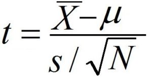
MedecialLabs001 makes a “Pill O” medicine that can control fever within 1.2 hours. A group of medical scientists created a “Pill N” with an entirely new chemical formula. They tested it on 100 people, and it could control fever for 1.05 hours with a typical variation from 0.5 hours. Now, the company’s CEO has to decide if it is worth launching “Pill N” in place of “Pill O”; for this, he has to ensure that the new medication is effective and that the difference in the mean isn’t due to chance.
Since we don’t have the entire population’s average deviation and only the sample standard deviation, we’ll run a one-sample T-test to conduct Hypothesis Testing and then calculate a t-score to determine the P-value.
First, we will decide on our Null Hypothesis that there is no distinction between the mean of the population and the sample average, i.e., H0 is m = x. Our Alternative Hypothesis, however, would suggest that the mean of the sample (time used to treat fever using “Pill N”) is lower than the mean of the population ( 1.2 hours), i.e., H1 = m > x. This is (as in Directional or The One Tail Hypothesis). A higher value, or even that there is an improvement in the mean of the samples, is useless for us since we know that a higher mean is a sure sign it is not a good thing. The new medication is not more effective than the prior one. Instead, we are most interested to find out whether the mean of the new drug is lower than the population means or not.
Then we will decide to set our significance level at 5 percent.
The t value is calculated by subtracting the sample’s mean from the population’s mean and then dividing it using the standard error Mean. The Standard Error of the Mean is computed by multiplying the sample size.
The t value is calculated as -3. The table for t-distribution only displays the P values for positive t values. To find out the p-value of an inverse t value, you simply need to find the p-value for its positive value. Calculate degrees of freedom, which in this case is N-1, i.e., 100-1=99. When we study the t-Table, we see that the t number is significant, and the variance between the sample and the mean of the sample is statistically significant. The crucial t value works out to 1.660 with a possibility that is P(m = x) = 0.00341551. Therefore, we deny the Null Hypothesis and state that the difference between the population’s mean and the sample’s mean is not due to chance but is rather statistically significant.
In previous blogs, if the sample size is sufficiently large, such as more than 30 people, then the gap between a Z-test and a t-Test isn’t that significant. We can show this. We assume that if the standard deviation of the population had been 0.5 hours, we could have had the ability to run a Z test. A Z Test’s value would also have been an obvious 3.
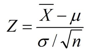
If we examine the z-table and calculate the p-value, it turns out as 0.0013. This is also because it is not high; we can reject our Null Hypothesis and are 99.87 percent certain of the fact that the Alternative Hypothesis is true.
Example 3
The median earnings of a student in the city “X” have typically been reported to be 45,000, with the standard deviation being 3000. An investigation was conducted on 120 graduates who work, and the median income was found as 47,000. Has the average income of graduates changed? Or is the fluctuation in the amount of money due to random chance?
In this case, we have to make a Null Hypothesis as being that there are no changes in the mean of the sample as well as the mean for the entire population; however, our alternative Hypothesis simply says that the sample mean is not the same as the mean of the population, i.e., H1 = M x.
In this case, we’ll use Z-test as the normal variation of the populace is known, and the distribution of the sample will be distributed normally (as there is a sample greater than).
But, interestingly enough, regardless of the p-value that we obtain from the z table, we’ll double it and then evaluate it against the significance threshold we have set, which is at the level of 5%. This is because, unlike the one-tailed alternative Hypothesis that looks at the data that is under the curve to either the left or the right of the sample mean, In a Two-Tailed Alternate Hypothesis, we look at both extremes. To further explain this, let’s first determine the Z-value.
In this case, the z-value would be 1.82 (45,000-45,500/3,000 (120)). (120)). If we look at this in a graphic way, when our significance was set at 5%, the meaning was that the left or rightmost five percent of the curve would represent our rejected region (depending on the kind of alternative hypotheses). If the value is the p-value, then we are able to disprove this as our Null Hypothesis. In this case, however, we will be able to say that our Acceptance Area will become in the middle, and our reject region of five percent will be divided between both sides, supplying 2.5 percent for each side in the distribution.
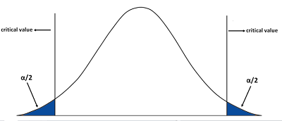
Then we can apply to use of the Table of Standard Probabilities for negative z scores to calculate the p-value of the left side on the right side of the line. To calculate this, let’s assume the z score to be negative. Therefore, the p-value of -1.82 is 0.0344. It is crucial to remember that we must find the p-value of both sides. To perform this, we can simply multiply the current p-value by two, i.e., 0.0344 x 2 = 0.0688. Our p-value is higher than the one we have proposed, so we are able to accept the Null Hypothesis says that there were not any statistically significant changes in income, and the variation in the mean of the sample is caused by random chance.
To comprehend this better, We can see that the median salary is 45,000, and even where the average deviation of 1.82, i.e., the salary is different from 1.82 Standard deviations, it does not include the figure of 45,500. The salary must have deviated from the standard deviation to arrive at this figure. Our significance at 5 percent, i.e., If a value of this magnitude is found in less than 20, it’s not due to chance. However, when the value is greater than one out of twenty, it is likely to be because of chance. The p-value, in this case, is estimated to be greater than 5 percent (i.e., greater than 0.05) which is why we conclude that the rise in the mean of our sample could be due to random chance.
Effect Size
We have already gone through a series of steps to determine the difference in the statistic of the sample and the population parameter and divide that variation with the standard error to determine the chance of getting this ratio from random chance (random sample error).
However, there is an error in this procedure, which involves the denominator. It has an important role, as the standard error across all denominators is less when the sample size is big, and the smaller the error of standard deviation, the greater the chances of it being statistically significant. Due to this, a tiny variance in the statistic of the sample and population parameter is considered to be statistically relevant (if your sample is sufficiently large).
So, for example, in the case of significant differences between the mean of the sample and the population mean, however, the size of the sample is 20, it could not be considered to be statistically significant, but the same difference would be considered significant when the sample size is 2000. Therefore, researchers are now focusing on both the statistical significance and the size of the effect.
Confidence Interval and Point Estimate
The two kinds of estimators include confidence Interval and Point Estimate, two forms of inferential statistics that give us insight that can be used to model or predictive analytics.
Confidence Interval
You’ve probably observed the use of confidence intervals within your day-to-everyday lives. They are among the most frequently utilized inferential statistics. Confidence intervals are utilized by researchers who are unable to determine the true populace parameter (population means). Therefore, we determine the confidence interval, which offers us the range of values that we can be confident to a certain extent that the range includes the population’s mean. To understand the concept better, take a look at the following examples.
Examples
Here are examples that can aid in understanding the way Confidence Interval functions.
Example 1
Let’s say the mean of the sample is 10. The Standard Deviation for the sample would be 2. Degrees of freedom are infinite (i.e., the amount of samples is many). We need to have a range of mean with a 95 percent and 99% confidence level.
The formula for calculating this will be
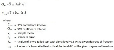
We now look at the table, and when df = a = .05, We can discover the t95 value to be 1.96.
CI95 = 10 +- (1.96)(.06)
CI95 = 10 +- .12
CI95 = 9.88, 10.12
So our range for the population’s mean comes from 9.88 to 10.12. 9.88 to 10.12 with 95% confidence.
For 99percent of us, the range will increase, i.e., to be more certain about our results.
CI99 = 10 +- (2.576)(.06)
CI99 = 10 +- .15
CI99 = 9.85, 10.15
Therefore, our range of the mean for the population is found to be 9.85 to 10.15. 9.85 to 10.15 with 99% certainty.
(Notice how the value of the minimum is reduced and the higher value gets increased)
Example 2
It is a sample of 36 (N=36). The average of this sample is 3.6. What is the meaning of the population?
In this case, we can employ an easy formula
M = x +/- SE
M = 25.5 + 3.636/(36)
M = 25.5 +/- 0.6
M = 24,9 to 26.1
Here, the confidence level is set at one std. We can see that for a normal distribution, the curvature’s area is 68.7; therefore, we can be 68.7 percent certain of this number. For a 95 percent confidence, i.e., two std, we divide this standard error by two.
M = 25.5 +/- 0.6 x 2
M = 25.5 +/- 1.2
M equals 24.3 to 26.7
Point Estimate
The point estimate is the process where we attempt to pinpoint the exact location of a statistic rather than giving an estimate of the number.
For example, The sample variance is an example of a point estimate. Any statistic can be a point estimate. One example could be estimating the average rainfall of Mumbai.
Knowing how hypothesis testing works, it is now possible to understand the different tests of statistical significance which can be employed to test hypotheses and make inferences from the data. The different statistical tests discussed in the following blog posts include T-Tests, F-Tests, and chi-square.


